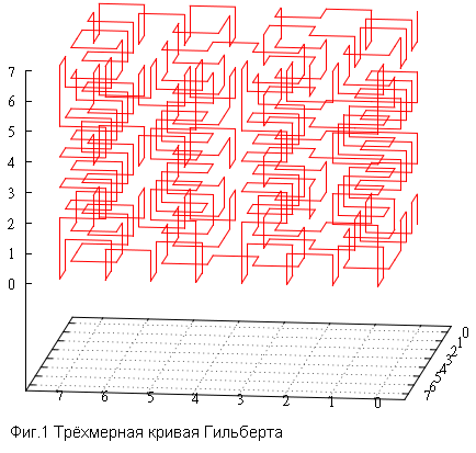
The Hilbert curve vs. Z-order

Repeatedly heard the opinion that of all swept curves. it the Hilbert curve the most promising for spatial indexing. The explanation given is that it does not contain discontinuities and therefore in some sense “well-arranged”. Whether so it actually and what is the spatial indexing, we will understand under the cut.

The concluding article of the series:

the

The Hilbert curve has the remarkable property — the distance between two successive points is always equal to one (step current of detail, to be precise). Therefore, data is not much different Hilbert curve values are close to each other (the inverse, incidentally, is wrong — adjacent points may be very different in meaning). For this property it is used, for example,

the

of dimension reduction (color palette)
improve locality of access in multidimensional indexing (here)
in the design of the antennas (SDAs)
clustering tables (DB2)

Regarding spatial data, the properties of the Hilbert curve allows to increase the locality of references and improve cache performance of a DBMS as SDAswhere the use table is recommended to Supplement the column with a calculated value and sort by this column.

In the spatial search, the Hilbert curve is present in Hilbert R-trees, where the basic idea (very roughly) — when it comes time to split the page in two descendants — sorted all items on the page according to the values of centroid and divide in half.

But we are more interested in another property of the Hilbert curve is self-similar curve is swept. So you can use it in the index-based B-tree. We are talking about the way of numbering of a discrete space.

the

Let you set discrete space of dimension N.
Assume also that we have some way of numbering all the points of this space.
Then, to index point feature enough to put in the index B-tree-based point numbers which hit these objects.
Search in this spatial index depends on the method of numbering and ultimately comes down to selection on the index of intervals of values.
sweep out curves good for its self-similarity, which allows to generate a relatively small number of such pointervalue, whereas other methods (for example, the similarity of the line scan) requires a huge number of subqueries, making such spatial indexing is ineffective.

So where does this intuitive sense that the Hilbert curve is good for spatial indexing? Yes, there are no breaks, the distance between any consecutive points is equal to the sampling rate. So what? What is the connection between this fact and the potentially high performance?
In the the beginning we have formulated a rule "good" method of ordering minimizes the total perimeter of the index pages. We are talking about B-tree pages, which in the end would be data. In other words, the performance index is determined by the number of pages that have to be read. The fewer pages, the average query reference size, the higher the (potential) performance of the index.

From this point of view, Hilbert's curve looks very promising. But it is the intuitive sense of bread will not smear, therefore undertake numerical experiment.

the

will consider 2 and 3 dimensional space
take the square/cube queries of different sizes
to a series of random queries of the same type and size calculate average/variance of the number of pages swept, in a series of 1000 requests

we proceed from the fact that each node of the space the point lies in. You can jot down random data and check on them, but then there would be questions about the quality of these random data. And so we have quite an objective measure of “fit”, though far from any real data set the

on the page is placed 200 items, it is important that it would not be a power of two, which would lead to vyrozhdennom case
compare between a Hilbert curve and Z-curve

That's how it looks in charts.

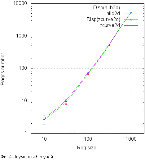
Now it should be at least out of curiosity to see how with a fixed request size (100X100 2D) behaves in the number of pages read, depending on the page size.

Clearly visible “hole” in Z-order corresponding to the size 128, 256 and 512. And the “holes” in 192, 384, 768. Are not that great.

As we can see, the difference can reach 10%, but almost everywhere is within statistical error. However, everywhere the Hilbert curve is better than the Z-curve. Not much, but better. Apparently, the 10% is the upper bound of the potential effect that can be achieved by clicking on the Hilbert curve. Is the game worth the candle? Try to find out.

the

Implementation.

Using Hilbert curve in the spatial search faces several challenges. For example, the key calculation of the 3 coordinates is (for the author) of about 1000 cycles is about 20 times more than the same for zcurve. Perhaps there is a more effective method in addition it is believed that the decrease in the number of pages read pays any complexity. Ie drive — more expensive resource than the processor. Therefore, we will primarily focus on the read buffer, and the time just take note.

With regard to algorithm search. Briefly, it is based on two main ideas:

Index is a B-tree with his paged. If we want to log access to the first element of extradition, should like a binary search to use the strategy of “divide and conquer”. Ie is needed for each iteration on average to equally divide the query into subqueries.

But unlike binary search in this case, the partition does not divide in half the number of disposable elements, and occurs according to a geometric principle.

Swept from the self-similarity of the curves it follows that if we take a square (cubic) lattice emerging from the origin in increments of powers of two, any elementary cube in the lattice contains one interval of values. Therefore, dissecting the search query to nodes of the lattice can break the original arbitrary subquery for continuous intervals. Then each of these intervals is deducted from the tree.

All this is equally true for the Hilbert curve and Z-order. However:

the

to the curve, Hilbert order has broken down — the lower left point of the query is not necessarily smaller than the right top (two dimensional case)

moreover, it is not necessarily a maximum and/or minimum of the subquery is in one of its corners, it is not all lies in the scope of the request the

consequently, this value range can be much wider search query in the worst case, the whole extent of the layer, if you managed to get into the area around the centre

This leads to the fact that it is necessary to modify the original algorithm.
First, change the interface of the key.

the

bitKey_limits_from_extent — this method is called once at the beginning of the search to determine the present boundaries of the search. The input receives the coordinates of the search extent, gives the minimum and maximum values of the searching range.

bitKey_getAttr — in the input accepts a range of values of the subquery and also the initial coordinates of the search query. Returns the mask of the following values

baSolid — the subquery lies entirely within the extent of the search, it should not be split, and can be values from interval be placed in the results

baReadReady minimum key spacing subquery lies within the search extent, you can do a search in the B-tree. In the case of zcurve this bit is always cocked.

baHasSmth — if this bit is not cocked, the subquery is entirely out of the search query and should be ignored. In the case of a Z-order this bit is always cocked.

The modified search algorithm looks like this:

set up a queue of subqueries, initially in the queue only one element — the extent (minimum and maximum key range), found by calling bitKey_limits_from_extent
While the queue is not empty:
1. Get the item from the top of the queue
2. Get information about it using the bitKey_getAttr
3. not armed baHasSmth, and ignore the subquery
4. cocked baSolid, deducted the entire range of values directly in resultset and go to the next subquery
5. cocked baReadReady, do a search in B-tree minimum value in the subquery
6. If it is not cocked or baReadReady for this request does not trigger the stopping criterion (it does not fit on one page)
  1. the Computed minimum and maximum values of the range of a subquery
  2. Find the category key which will be cut
  3. there are two subquery
  4. and Put them into a queue, first one with large values, then the second

Consider the example query in the extent [...524000,0,484000 525000,1000,485000].

Here is the execution of the request for Z-order, nothing more.
Subqueries — all generated subqueries results — found points,
lookups requests to the B-tree.

Since the range crosses 0x80000, the starting extent size is obtained in the entire extent of the layer. All the fun is merged into the center, consider in more detail.

Draw attention to "clusters" of subqueries on the borders. The mechanism of their formation is something like this — say, a cut the compartment from the perimeter of the search extent of the narrow strip, for example, a width of 3. Moreover, in this strip even no periods, but we do not know. A check can only in the moment when the minimum value of the range of the subquery fall within the search extent. As a result, the algorithm will cut the strip down to subqueries of size 2 and 1, and only then will be able to make a request to the index to make sure there's nothing there. Or so.
The number of pages read is not affected, all such passages In the tree have the cache, but the amount of work done is impressive.

Well, we have to figure out how much was actually read and how much time it all took. The following values are obtained on the same data in the same way that previously. I.e. 100 000 000 random points in the [0...1 000 000, 0...0, 0...1 000 000].

The measurements were carried out on a modest virtual machine with two cores and 4 GB of RAM, so the times are not absolute values, but the numbers of pages read is still possible to trust.

The times shown in the second runs, on a heated server and virtual machine. The number of read buffers — into the fresh-raised server.
the the the the the the the the

NPoints	Nreq	Type	Time(ms)	Reads	Hits
1	100 000	zcurve rtree hilbert	.36 .38 .63	1.13307 1.83092 1.16946	3.89143 3.84164 88.9128
10	100 000	zcurve rtree hilbert	.38 .46 .80	1.57692 2.73515 1.61474	7.96261 4.35017 209.52
100	100 000	zcurve rtree hilbert	.48 .50 ... 7.1 * 1.4	3.30305 6.2594 3.24432	31.0239 4.9118 465.706
1 000	100 000	zcurve rtree hilbert	1.2 1.1 ... 16 * 3.8	13.0646 24.38 11.761	165.853 7.89025 1357.53
10 000	10 000	zcurve rtree hilbert	5.5 4.2 ... 135 * 14	65.1069 150.579 59.229	651.405 27.2181 4108.42
100 000	10 000	zcurve rtree hilbert	53.3 35...1200 * 89	442.628 1243.64 424.51	2198.11 186.457 12807.4
1 000 000	1 000	zcurve rtree hilbert	390 ...10000 300* 545	3629.49 11394 3491.37	6792.26 3175.36 36245.5

where
Npoints — the average number of points in the results
Nreq — the number of queries in the series
Type — ‘zcurve’ — fixed algorithm with hypercube and numeric analysis using its internal structure;’rtree’- gist only 2D rtree; ‘hilbert’ is the same algorithm as for the zcurve, but by the Hilbert curve, (*) — in order to compare search time was needed to adjust the series 10 times in order to pages fit in the cache
Time(ms) — average time of query execution
Reads — the average number of readings per request. the Most important column.
Shared hits — the number of accesses to the buffers

* — the spread of values is due to the high instability of the results, if the buffer was successfully found in the cache, it was observed first, in the case of massive failures is the second. In fact, the second number is typical for the claimed Nreq, the first — 5-10 times smaller.

the

Insights

A little surprised that the small ad-rating benefits by the Hilbert curve gave a rather accurate assessment of the real situation.

It is seen that for queries in which the size of the issue comparable with or more than the page size, the Hilbert curve starts to behave better in the number of misses by the cache. Winning, however, of a few percent.

On the other hand, the integral time for the Hilbert curve is approximately twice worse thereof in the Z-curve. For example, the author chose not the most efficient method of calculating the curve, for example, something could be done more careful. But the calculation of the Hilbert curve is objectively heavier than the Z-curve to work with it really need to take significantly more action. The feeling is that to play it slow with a few percent gain in reading of pages fail.

Yes, we can say that in a highly competitive environment each reading page is more expensive tens of thousands of computing key. But the number of successful cache hits have by the Hilbert curve significantly more, and they pass through the serialization, and in a competitive environment is also worth something.

the

total

That brings me to the end of the epic narrative about the capabilities and features of spatial and/or multidimensional indexes based on self-similar swept curves, built on B-trees.

During this time (except that implementing such an index), we found that compared with traditionally used in this area, R-tree
the

it is more compact (objectively better average occupancy of pages)
faster builds
does not use heuristics (i.e., it is the algorithm)
not afraid of dynamic changes
for small and medium-sized queries running faster.
Loses on large queries (just in excess of memory for the page cache) where the issuance involves hundreds of pages.
While R-tree is faster because filtering happens only on the perimeter, the treatment of which swept curves noticeably heavier.
Under normal conditions, competition for memory and for such queries, our index is considerably faster than R-tree.
Without changing the algorithm works with keys of any (reasonable) dimensions
it is possible to use heterogeneous data in a single key, for example, time, object class and coordinates. It does not have to configure any of the heuristics in the worst case, if the data ranges varies greatly will drop performance.
features ((multidimensional) intervals) are interpreted as points, spatial semantics is handled within the boundaries of the search extents.
allowed the mixing of interval and accurate data in a single key, again all semantics shall be made out, the algorithm is not changed

All this does not require any SQL syntax, the introduction of new types ...
If you want, you can write a wrapping extension for PostgreSQL. the

And Yes, lined under the BSD license, allowing almost complete freedom of action.

Article based on information from habrahabr.ru

Поиск по этому блогу

computer express